Sections

Learning Objectives Graphing Velocity as a Function of Time Solving Problems using Velocity–Time Graphs Practice Problems Check Your Understanding

Learning Objectives

By the end of this section, you will be able to do the following:

Explain the meaning of slope and area in velocity vs. time graphs
Solve problems using velocity vs. time graphs

Section Key Terms
acceleration

Graphing Velocity as a Function of Time

Earlier, we examined graphs of position versus time. Now, we are going to build on that information as we look at graphs of velocity vs. time. Velocity is the rate of change of displacement. Acceleration is the rate of change of velocity; we will discuss acceleration more in another chapter. These concepts are all very interrelated.

Virtual Physics

Maze Game

In this simulation you will use a vector diagram to manipulate a ball into a certain location without hitting a wall. You can manipulate the ball directly with position or by changing its velocity. Explore how these factors change the motion. If you would like, you can put it on the a setting, as well. This is acceleration, which measures the rate of change of velocity. We will explore acceleration in more detail later, but it might be interesting to take a look at it here.

In this game, students will use a vector arrow to explore position and velocity. The task is to get a ball into the pinpointed location without it hitting a wall.

Figure 2.17 Click here for the simulation

Grasp Check

In which setting, displacement or velocity, can the ball be easily manipulated and why?

The ball can be easily manipulated with displacement because the arena is a position space.
The ball can be easily manipulated with velocity because the arena is a position space.
The ball can be easily manipulated with displacement because the arena is a velocity space.
The ball can be easily manipulated with velocity because the arena is a velocity space.

What can we learn about motion by looking at velocity vs. time graphs? Let’s return to our drive to school, and look at a graph of position versus time as shown in Figure 2.18.

A line graph titled Position versus Time is shown. The x-axis is labeled time in minutes and has a scale from zero to twenty in increments of one. The y-axis is labeled position, d, in kilometers and has a scale from zero to twelve in increments of one. The line intersects the following data points to form a line that slopes upward and then downward: zero, zero; two, one; four, two; ten, five; twelve, four; fourteen, three; twenty, zero.

Figure 2.18 A graph of position versus time for the drive to and from school is shown.

We assumed for our original calculation that your parent drove with a constant velocity to and from school. We now know that the car could not have gone from rest to a constant velocity without speeding up. So the actual graph would be curved on either end, but let’s make the same approximation as we did then, anyway.

Tips For Success

It is common in physics, especially at the early learning stages, for certain things to be neglected, as we see here. This is because it makes the concept clearer or the calculation easier. Practicing physicists use these kinds of short-cuts, as well. It works out because usually the thing being neglected is small enough that it does not significantly affect the answer. In the earlier example, the amount of time it takes the car to speed up and reach its cruising velocity is very small compared to the total time traveled.

Looking at this graph, and given what we learned, we can see that there are two distinct periods to the car’s motion—the way to school and the way back. The average velocity for the drive to school is 0.5 km/minute. We can see that the average velocity for the drive back is –0.5 km/minute. If we plot the data showing velocity versus time, we get another graph (Figure 2.19):

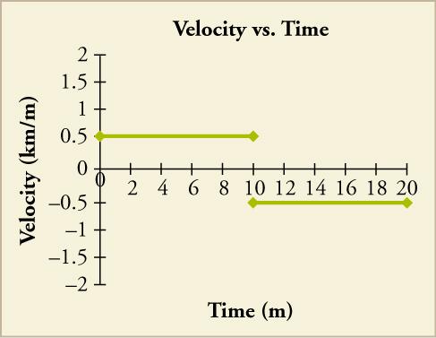
A graph that shows time in minutes on the x-axis and velocity in kilometers per minute on the y axis. A horizontal line is show at a velocity of 0.5 that runs from 0 to 10 minutes. Another horizontal line is shown at a velocity of –0.5 that runs from 10 to 20 minutes.

Figure 2.19 Graph of velocity versus time for the drive to and from school.

We can learn a few things. First, we can derive a v versus t graph from a d versus t graph. Second, if we have a straight-line position–time graph that is positively or negatively sloped, it will yield a horizontal velocity graph. There are a few other interesting things to note. Just as we could use a position vs. time graph to determine velocity, we can use a velocity vs. time graph to determine position. We know that v = d/t. If we use a little algebra to re-arrange the equation, we see that d = v $\times$ t. In Figure 2.19, we have velocity on the y-axis and time along the x-axis. Let’s take just the first half of the motion. We get 0.5 km/minute $\times$ 10 minutes. The units for minutes cancel each other, and we get 5 km, which is the displacement for the trip to school. If we calculate the same for the return trip, we get –5 km. If we add them together, we see that the net displacement for the whole trip is 0 km, which it should be because we started and ended at the same place.

Tips For Success

You can treat units just like you treat numbers, so a km/km=1 (or, we say, it cancels out). This is good because it can tell us whether or not we have calculated everything with the correct units. For instance, if we end up with m × s for velocity instead of m/s, we know that something has gone wrong, and we need to check our math. This process is called dimensional analysis, and it is one of the best ways to check if your math makes sense in physics.

The area under a velocity curve represents the displacement. The velocity curve also tells us whether the car is speeding up. In our earlier example, we stated that the velocity was constant. So, the car is not speeding up. Graphically, you can see that the slope of these two lines is 0. This slope tells us that the car is not speeding up, or accelerating. We will do more with this information in a later chapter. For now, just remember that the area under the graph and the slope are the two important parts of the graph. Just like we could define a linear equation for the motion in a position vs. time graph, we can also define one for a velocity vs. time graph. As we said, the slope equals the acceleration, a. And in this graph, the y-intercept is v₀. Thus, $v = v_{0} + a t$ .

But what if the velocity is not constant? Let’s look back at our jet-car example. At the beginning of the motion, as the car is speeding up, we saw that its position is a curve, as shown in Figure 2.20.

A line graph titled Jet Car Displacement is shown. The x-axis is labeled time, t, in seconds and has a scale from zero to forty on increments of ten. The y-axis is labeled displacement, x, in meters and has a scale from zero to three thousand five hundred in increments of five hundred. The following approximate data points are plotted, resulting in a line that curves upward: eight, two hundred fifty; ten, five hundred; fifteen, one thousand; twenty, one thousand five hundred; twenty-five, two thousand; th

Figure 2.20 A graph is shown of the position of a jet-powered car during the time span when it is speeding up. The slope of a d vs. t graph is velocity. This is shown at two points. Instantaneous velocity at any point is the slope of the tangent at that point.

You do not have to do this, but you could, theoretically, take the instantaneous velocity at each point on this graph. If you did, you would get Figure 2.21, which is just a straight line with a positive slope.

A line graph titled Jet Car Velocity is shown. The x-axis is labeled time, t, in seconds and has a scale from zero to forty on increments of ten. The y-axis is labeled velocity, v, in meters per second and has a scale from zero to one hundred eighty in increments of twenty. A straight line with a positive slope is plotted that intersects the following approximate points: zero, eighteen; ten, sixty (labeled P); fifteen, ninety; twenty, one hundred twenty; twenty five, one hundred fifty (labeled Q); thirty,

Figure 2.21 The graph shows the velocity of a jet-powered car during the time span when it is speeding up.

Again, if we take the slope of the velocity vs. time graph, we get the acceleration, the rate of change of the velocity. And, if we take the area under the slope, we get back to the displacement.

Solving Problems using Velocity–Time Graphs

Most velocity vs. time graphs will be straight lines. When this is the case, our calculations are fairly simple.

Worked Example

Using Velocity Graph to Calculate Some Stuff: Jet Car

Use this figure to (a) find the displacement of the jet car over the time shown (b) calculate the rate of change (acceleration) of the velocity. (c) give the instantaneous velocity at 5 s, and (d) calculate the average velocity over the interval shown.

Strategy

The displacement is given by finding the area under the line in the velocity vs. time graph.
The acceleration is given by finding the slope of the velocity graph.
The instantaneous velocity can just be read off of the graph.
To find the average velocity, recall that $v_{avg} = \frac{Δ d}{Δ t} = \frac{d_{f} - d_{0}}{t_{f} - t_{0}}$

Solution

1. Analyze the shape of the area to be calculated. In this case, the area is made up of a rectangle between 0 and 20 m/s stretching to 30 s. The area of a rectangle is length $\times$ width. Therefore, the area of this piece is 600 m.
2. Above that is a triangle whose base is 30 s and height is 140 m/s. The area of a triangle is 0.5 $\times$ length $\times$ width. The area of this piece, therefore, is 2,100 m.
3. Add them together to get a net displacement of 2,700 m.
1. Take two points on the velocity line. Say, t = 5 s and t = 25 s. At t = 5 s, the value of v = 40 m/s.
  
  At t = 25 s, v = 140 m/s.
2. Find the slope. $\begin{matrix} a & = & \frac{Δ v}{Δ t} \\ = & \frac{100 m/s}{20 s} \\ = & 5 {m/s}^{2} \end{matrix}$
The instantaneous velocity at t = 5 s , as we found in part (b) is just 40 m/s.
1. Find the net displacement, which we found in part (a) was 2,700 m.
2. Find the total time which for this case is 30 s.
3. Divide 2,700 m/30 s = 90 m/s.

Discussion

The average velocity we calculated here makes sense if we look at the graph. 100m/s falls about halfway across the graph and since it is a straight line, we would expect about half the velocity to be above and half below.

Tips For Success

You can have negative position, velocity, and acceleration on a graph that describes the way the object is moving. You should never see a graph with negative time on an axis. Why?

Most of the velocity vs. time graphs we will look at will be simple to interpret. Occasionally, we will look at curved graphs of velocity vs. time. More often, these curved graphs occur when something is speeding up, often from rest. Let’s look back at a more realistic velocity vs. time graph of the jet car’s motion that takes this speeding up stage into account.

A line graph titled Jet Car Velocity is shown. The x-axis is labeled time, t, in seconds and has a scale from zero to eighty on increments of ten. The y-axis is labeled velocity, v, in meters per second and has a scale from one hundred sixty to two hundred sixty in increments of ten. The following approximate data points are plotted and connected to form a line that curves upward, and then becomes flat: zero, one hundred sixty five; ten, two hundred ten; twenty, two hundred thirty; thirty, two hundred for

Figure 2.22 The graph shows a more accurate graph of the velocity of a jet-powered car during the time span when it is speeding up.

Worked Example

Using Curvy Velocity Graph to Calculate Some Stuff: jet car, Take Two

Use Figure 2.22 to (a) find the approximate displacement of the jet car over the time shown, (b) calculate the instantaneous acceleration at t = 30 s, (c) find the instantaneous velocity at 30 s, and (d) calculate the approximate average velocity over the interval shown.

Strategy

Because this graph is an undefined curve, we have to estimate shapes over smaller intervals in order to find the areas.
Like when we were working with a curved displacement graph, we will need to take a tangent line at the instant we are interested and use that to calculate the instantaneous acceleration.
The instantaneous velocity can still be read off of the graph.
We will find the average velocity the same way we did in the previous example.

Solution

1. This problem is more complicated than the last example. To get a good estimate, we should probably break the curve into four sections. 0 → 10 s, 10 → 20 s, 20 → 40 s, and 40 → 70 s.
2. Calculate the bottom rectangle (common to all pieces). 165 m/s $\times$ 70 s = 11,550 m.
3. Estimate a triangle at the top, and calculate the area for each section. Section 1 = 225 m; section 2 = 100 m + 450 m = 550 m; section 3 = 150 m + 1,300 m = 1,450 m; section 4 = 2,550 m.
4. Add them together to get a net displacement of 16,325 m.
Using the tangent line given, we find that the slope is 1 m/s².
The instantaneous velocity at t = 30 s, is 240 m/s.
1. Find the net displacement, which we found in part (a), was 16,325 m.
2. Find the total time, which for this case is 70 s.
3. Divide $\frac{16,325 m}{70 s} \sim 233 m/s$

Discussion

This is a much more complicated process than the first problem. If we were to use these estimates to come up with the average velocity over just the first 30 s we would get about 191 m/s. By approximating that curve with a line, we get an average velocity of 202.5 m/s. Depending on our purposes and how precise an answer we need, sometimes calling a curve a straight line is a worthwhile approximation.

Practice Problems

4e5ce2cc9504dcbc01236ff37b443e0bd8a93ae5

Figure 2.23

Consider the velocity vs. time graph shown below of a person in an elevator. Suppose the elevator is initially at rest. It then speeds up for 3 seconds, maintains that velocity for 15 seconds, then slows down for 5 seconds until it stops. Find the instantaneous velocity at t = 10 s and t = 23 s.

Instantaneous velocity at t = 10 s and t = 23 s are 0 m/s and 0 m/s.
Instantaneous velocity at t = 10 s and t = 23 s are 0 m/s and 3 m/s.
Instantaneous velocity at t = 10 s and t = 23 s are 3 m/s and 0 m/s.
Instantaneous velocity at t = 10 s and t = 23 s are 3 m/s and 1.5 m/s.

Figure 2.24

Calculate the net displacement and the average velocity of the elevator over the time interval shown.

Net displacement is 45 m and average velocity is 2.10 m/s.
Net displacement is 45 m and average velocity is 2.28 m/s.
Net displacement is 57 m and average velocity is 2.66 m/s.
Net displacement is 57 m and average velocity is 2.48 m/s.

Snap Lab

Graphing Motion, Take Two

In this activity, you will graph a moving ball’s velocity vs. time.

Materials

your graph from the earlier Graphing Motion Snap Lab!
1 piece of graph paper
1 pencil

Procedure

Take your graph from the earlier Graphing Motion Snap Lab! and use it to create a graph of velocity vs. time.
Use your graph to calculate the displacement.

Grasp Check

Describe the graph and explain what it means in terms of velocity and acceleration.

The graph shows a horizontal line indicating that the ball moved with a constant velocity, that is, it was not accelerating.
The graph shows a horizontal line indicating that the ball moved with a constant velocity, that is, it was accelerating.
The graph shows a horizontal line indicating that the ball moved with a variable velocity, that is, it was not accelerating.
The graph shows a horizontal line indicating that the ball moved with a variable velocity, that is, it was accelerating.

Check Your Understanding

Exercise 11

What information could you obtain by looking at a velocity vs. time graph?

acceleration
direction of motion
reference frame of the motion
shortest path

Exercise 12

How would you use a position vs. time graph to construct a velocity vs. time graph and vice versa?

Slope of position vs. time curve is used to construct velocity vs. time curve, and slope of velocity vs. time curve is used to construct position vs. time curve.
Slope of position vs. time curve is used to construct velocity vs. time curve, and area of velocity vs. time curve is used to construct position vs. time curve.
Area of position vs. time curve is used to construct velocity vs. time curve, and slope of velocity vs. time curve is used to construct position vs. time curve.
Area of position/time curve is used to construct velocity vs. time curve, and area of velocity vs. time curve is used to construct position vs. time curve.

2.4 Velocity vs. Time Graphs

Learning Objectives